1. Introduction
1.1. Before you start
In the following we assume that you, the reader, has a general familiarity with optimization methods. You should be very well familiar with linear systems of equations and be aware of issues when they are over- oder under-determined, and the basics of inverse problems. You should know what a Tikhonov-Philips functional is, how this can be solved numerically using the Landweber method. You should be familiar with Hilbert spaces and know the principal differences to more general Banach spaces.
If you are not familiar with the above terminology, then we recommend an introductory book to regularization methods such as [Schuster2012]. However, a small introduction is also given in [background].
If you are generally interested in the mathematical background of Banach spaces, Bregman distances and so on, we recommend [Cioranescu1990].
1.2. What is BASSO?
BASSO is a library written in C++ to solve inverse problems in Banach spaces. It is both an interface in C++ and in Python3. Moreover, it comes with a bunch of tools that allow to address certain kind of inverse problems, e.g. inverse problems of ill-conditioned matrices, matrix factorization and certain specific classical inverse problems such as Computerized Tomography. These also may serve as examples how to use the library.
We stress that the library’s interface is written from the viewpoint of the mathematical objects encountered in this problem setup, i.e. there are classes that model vector spaces, normed vector spaces and elements thereof. There are mappings between spaces and functions working on elements from specific spaces. In order to put these to their best use it is recommended to have a background of the mathematical concepts involved.
Therefore, it is not aimed at users who simply wish to call a function to solve a certain type of inverse problem although it comes with a few helper programs that might do the job. At its core it is a library that allows to solve an inverse problem if ones possesses some knowledge of the mathematical underpinning and wishes to see this at work. Extensive care has been taken such that the library automatically prevents mishaps in the tool development such as using vectors from the "wrong" space, use mappings in the wrong way, and so on.
1.3. Installation
In the following we explain the installation procedure to get BASSO up and running.
1.3.1. Installation requirements
This program suite is implemented using C++ and Python3 and the development mainly focused on Linux (development machine used Ubuntu 14.04 and 16.04). At the moment other operating systems are not supported but may still work. Note that the build system depends on CMake which principally allows to generate configuration files also for Integrated Developer Environments popular on Windows.
It has the following non-trivial dependencies:
Note that these packages can be easily installed using either the repository tool (using some linux distribution such as Ubuntu), e.g.
sudo apt install cmake
Moreover, the following packages are not ultimately required but examples or tests may depend on them:
1.3.2. Installation procedure
Installation comes in two flavors: either via a tarball or a cloned repository.
The tarball releases are recommended if you only plan to use BASSO and do not intend modifying its code. If, however, you need to use a development branch, then you have to clone from the repository.
In general, this package is compiled and installed via CMake. Please refer to the text README file that is included in the tarball.
1.3.3. From Tarball
Unpack the archive, assuming its suffix is .gz.
tar -zxvf basso-${revnumber}.tar.gz
1.3.4. From cloned repository
In case you are cloning the repository,
git clone https://github.com/FrederikHeber/BASSO.git
then you are in the same position as having unpacked the release tarball.
Enter the directory
cd basso
Continue then in section Configure, make, install.
1.3.5. Configure, make, make install
Next, we recommend to build the toolkit not in the source folder but in an extra folder, e.g., “build64”. This is called an out-of-source build. It prevents cluttering of the source folder. Naturally, you may pick any name (and actually any location on your computer) as you see fit.
mkdir build64
cd build64
cmake ..
make
make install
|
Important
|
There are many options to control cmake, e.g. giving a prefix to set the installation location, directing to unusually installed boost or eigen versions, and many more. For more details on these options with cmake please take a look at the up-to-date README` file |
|
Note
|
We recommend executing (after make install was run) make -j4 test additionally. This will execute every test on the extensive testsuite and report any errors. None should fail. If all fail, a possible cause might be a not working tensorflow installation. If some fail, please contact the author. The extra argument -j4 instructs make to use four threads in parallel for testing. Use as many as you have cores on your machine. |
1.4. License
As long as no other license statement is given, ThermodynamicAnalyticsToolkit is free for use under the GNU Public License (GPL) Version 2 (see https://www.gnu.org/licenses/gpl-2.0.en.html for full text).
1.5. Disclaimer
Because the program is licensed free of charge, there is not warranty for the program, to the extent permitted by applicable law. Except when otherwise stated in writing in the copyright holders and/or other parties provide the program "as is" without warranty of any kind, either expressed or implied. Including, but not limited to, the implied warranties of merchantability and fitness for a particular purpose. The entire risk as to the quality and performance of the program is with you. Should the program prove defective, you assume the cost of all necessary servicing, repair, or correction.
— section 11 of the GPLv2 license
1.6. Feedback
If you encounter any bugs, errors, or would like to submit feature request, please open an issue at GitHub or write to frederik.heber@gmail.com. The authors are especially thankful for any description of all related events prior to occurrence of the error and auxiliary files. More explicitly, the following information is crucial in enabling assistance:
-
operating system and version, e.g., Ubuntu 16.04
-
BASSO version (or respective branch on GitHub), e.g., BASSO 1.10
-
steps that lead to the error, possibly with sample C++/Python code
Please mind sensible space restrictions of email attachments.
2. Background
One of the most ubiquitous tasks in computing is solving linear systems of equations, $A x = y$ where a matrix $A$ and a right-hand side vector $y$ are given and we are looking for the solution vector $x$. Because of the omnipresence of this problem, many different solution methods exist, whose applicability depends on the properties of the matrix: when the matrix is symmetric, one might use Cholesky factorization. If the matrix is symmetric and positive definite, and especially if it is very large, Conjugate Gradient schemes are typically employed.
If the matrix is generic, e.g., it is not symmetric, then more general schemes are necessary.
From a more mathematical perspective, $x$ is the element of a vector space $\mathrm{X}$. Moreover, the matrix is a linear operator mapping between this space $\mathrm{X}$ and and itself or maybe even another space $\mathrm{Y}$ that contains the given right-hand side $y$.
We are looking at the more interesting cases, where there is either no solution $x$ or infinitely many, i.e., the system is over- oder under-determined with a non-unique solution. Then, in order to define a "closest" solution in the sense $||Ax-y||$, we need norms that induce a metric. Therefore, the vector spaces are normed vector spaces.
When the row and column dimensions are not the same, then we certainly do not have a single space, but two spaces. This is also the case when different norms apply to source and target space. Moreover, when the norm is not an $\ell_2$-norm, then $\mathrm{X}$ is not even a Hilbert space.
With an under-determined or over-determined system of equation the linear operator is in general not invertible. The remedy is called regularization where the linear operator is modified in such a way as to become invertible but still as faithful as possible to its original version. More generally, regularization is required if the right-hand side is not in the range of the operator. This may also occur for the case of "noisy data", i.e., when the right-hand side $\widetilde{y} = y + \delta y$ is perturbed by white-noise $\delta y$.
Typically, (Tikhonov-)regularization is formulated as a minimization problem of a functional $F(x)$ by adding a penalty term as follows:
$min_x ( || Ax-y ||^2 + \lambda ||x||^2) =: min_x F(x)$.
This minimization problems contains two terms: the first is called the data fidelity term that minimizes the residual, i.e. the metric distance to the sets of admissible solutions. The second term is the regularization term that enforces a minimum-norm solution.
Through the minimum norm requirement a solution can be sought that is equipped with certain favorable properties. For example, a sparse solution is obtained of the $\ell_1$-norm is used.
As already mentioned, depending on the employed norms in this minimization problem, the solutions no longer live in a Hilbert space but in a more general Banach space, e.g., the N-dimensional vector space $\mathrm{R}^N$ equipped with the norm \ell_{1.1} norm. Convergence theoretical results are well-established for Hilbert spaces. For Banach spaces the situation is more difficult: In a Banach space the space and its dual do not in general coincide, namely they are not in general isometric isomorphic to each other.
This in turn causes us to deal not with two spaces, $\mathrm{X}$ and $\mathrm{Y}$, but with possibly up to four spaces, $\mathrm{X}$, $\mathrm{X}^\ast$, $\mathrm{Y}$, and $\mathrm{Y}^\ast$.
What is the relation between those spaces? Let us give a figure of the mappings.
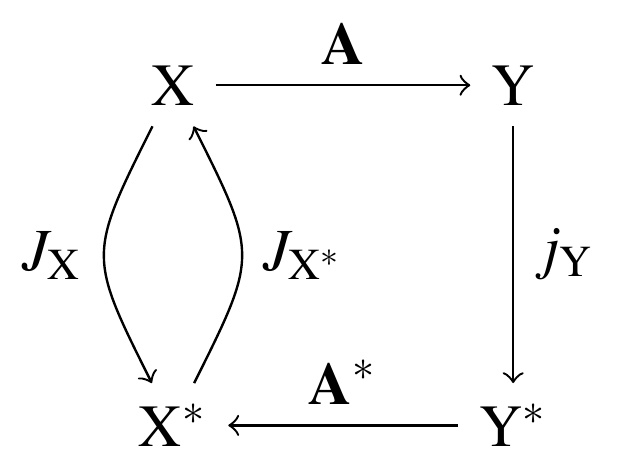
The matrix $A$ and its dual mapping $A^\ast$, which in finite dimensions is simply the complex conjugate, are obvious. However, what are $J_p$ and so forth?
The residual $Ax-y$ gives us the natural direction of error as the only information we have about the true solution $x$ is given in the mapped form as the right-hand side $y$. Therefore, we need a mapping that preserves angles and lengths with respect to the norm of the respective space. This role is fulfilled by the so-called duality mappings
$J_p = { x^\ast \in \mathrm{X}^\ast | <x^\ast, x> = ||x||^p_{\mathrm{X}}, ||x^\ast|| = ||x||^{p-1} }$,
where p is associated with the gauge function $t \rightarrow t^{p-1}$.
[In lp-spaces these two p coincide.]
These are connected to the (sub-)gradient of the norm through the famous theorem of Asplund, $J_p(x) = \frac{\partial}{\partial x} ( \frac 1 p ||x||^p)$
A sub-gradient is a generalization of the gradient where the space is no longer smooth and therefore the gradient is no longer unique.
As last but one ingredient we need a new distance measure, replacing the metric distance that has failed so far in allowing a proof of convergence. We use the Bregman distance,
$\Delta(x,y) = \tfrac 1 {p^\ast} ||x||^p - < J_p (x), y > + \frac 1 p || y ||^p$
Finally, we seek for iterative solutions for the above minimization functional, i.e., we have a procedure $x_{n+1} = x_n + f(x_n, \Delta F(x_n))$, where the current iterature $x_n$ and the gradient of the functional to be minimized $F(x_n)$, see above, are used to obtain the next iterate $x_{n+1}$.
In case of noisy right-hand sides, when no exact solution exists, the iteration with respect to the minimization functional shows a typical behavior (assuming we start with the origin as the first iterate): The data fidelity term decreases and the minimum-norm term increases. There is a cross-over point where the sum of the two no longer decrease but increases because the minimum-norm term dominates. This gives rise to a so-called "L"- shape and requires a stopping rule for the minimization as the optimal solution lies at the kink of the L. This is called semi-convergence.
All of this can be found in the following nice-to-read academical papers:
-
First paper on a non-linear Landweber method using Duality Mappings for general smooth, convex Banach spaces. Proof of strong convergence in noise-free case.
-
Paper on the underlying relation between Metric and Bregman projections that form the essential basis for the Sequential Subspace Methods. Multiple search directions. Proof of weak convergence.
-
Extension to perturbed right-hand sides. Proof of strong convergence for specific set of multiple search directions. Fast method when using two search directions by projection onto hyperplanes.
-
[Heber2019] (also available as arXiv preprint [Heber2016]).
Acceleration of the Sequential Subspace Methods by using metric projections to orthogonalize search directions. Connection to Conjugate Gradient Minimal Error method.
If you want to constrain yourself to a single paper, then we recommend the last one as it formed the basis for this library.
3. Overview
This mathematical introduction is necessary to understand the following elements contained in this library and put them to the best possible use.
Note that although the primary interface is written in C++, there is also a Python 3 interface. However, in this section we only go over the primary interface classes. The python interface is discussed in a separate [python].
3.1. The Basic Elements
BASSO mimics all of these objects we have introduced before in its class structure:
-
(normed) vector space classes NormedSpace and NormedDualSpace,
-
norm class L1Norm, LpNorm, and LInfinityNorm,
-
vector class SpaceElement,
-
mapping classes DualityMapping — with specializations LpDualityMapping, L1DualityMapping, LInfinityDualityMapping — LinearMapping (for matrices), and TwoFactorLinearMapping (for product of two matrices used in factorization problems),
-
function(al) classes/functors such as BregmanDistance, ResidualFunctional, SmoothnessFunctional.
These can be considered the basic elements.
|
Note
|
BASSO is based on the well-known Eigen library for all linear algebra-relates routines. Therefore it uses the Eigen classes Eigen::MatrixXd and Eigen::VectorXd for representing vectors and matrices. |
3.2. Inverse problem and Solver classes
Moreover, it contains some more complex classes that comprise the linear system of equations to be solved or the overall problem structure, InverseProblem.
In order to solve this inverse problem of Ax=y we need solvers. Their classes are called LandweberMinimizer, SequentialSubspaceMinimizer or SequentialSubspaceMinimizerNoise (with additional noise in the right-hand side taken into account).
3.3. General usage concepts
Specific instances of these classes, e.g., the NormedSpace class, are created using the so-called Factory pattern by classes that typically share the same name just with an added Factory, e.g., NormedSpaceFactory. These contain a function create() that is called with certain parameters and returns a pointer to the created instance.
|
Important
|
All these pointers are wrapped into boost::shared_ptr to prevent memory loss, i.e. they deallocate automatically when the last reference to the pointer is no longer held. |
All things associated to an object, e.g., the norm of a space, can be queried from an instance using getters, e.g., NomedSpace.getNorm() for the norm, NormedSpace.getDimension() for the number of degrees of freedom of this space, or NormedSpace.getDualSpace() for its dual space. See [reference.NormedSpace] for details.
3.4. Rough sketch of inverse problem solving
The following should give you a rough idea of how to solve an inverse problem
-
Create the two Banach spaces as NormedSpace by supplying the respective lp norm parameter. Their dual spaces are created automatically and so are in turn the required duality mappings.
-
Create the right-hand side y as a SpaceElement by using NormedSpace.createElement() or ElementCreator.create() giving the associated space and the Eigen vector.
-
Create the linear mapping A using LinearMappingFactory.createInstance() giving the two spaces and the Eigen matrix.
-
Create the inverse problem InverseProblem giving the mapping, the two spaces and the right-hand side.
-
Create sensible starting values in the solution space and its dual. Note that zero is always an admissible starting value.
-
Finally, instantiate a solver such as SequentialSubspaceMinimizer give it the inverse problem, starting value and dual starting value and a true solution if known.
The result will be a structure wherein the approximate solution and a few other instances such as the residual or the number of iterations and the status are contained.
The first four steps can be combined using InverseProblemFactory that takes certain string arguments describing the spaces and the right-hand side and the matrix in Eigen-format.
This is the approach used in the Basso tool that ships with this library, see [examples.basso]
3.5. Inverse Problems with auxiliary constraints
For more complex problems a split feasibility ansatz is used where each constraint is fulfilled in turn in an iterative fashion. In other words, there are two iterations: An inner loop where the inverse problem is solved and an outer loop where the different parts of the split feasibility problem — the inverse problem is one of them — are minimized in turn.
To this end, there is the abstract FeasibilityProblem class, the AuxiliaryConstraintsProblem which combines it with an arbitrary combination of AuxiliaryConstraints such as unity, non-negativity or a logical combination of these. Finally, there is the high-level class SplitFeasibilitySolver that solves inverse problems with these additional auxiliary constraints. These constraints are simply `register()`ed with this class. See [reference.solvers.SplitFeasibilitySolver] for details.
Let us now look at an example where we solve the random matrix toy problem. We create a random matrix and a random right-hand side. We make sure that the right-hand side is actually in the range of the matrix. We construct all instances necessary for the solver and finally solve the inverse problem.
We look at two versions: First, we inspect the "long" version where most of the ingredients are set up by hand. There you will see all of the basic elements that we talked about before. In the second "short" version we will use a lot of convenience objects.
|
Note
|
We hide away all includes and two static functions for creating a random vector and a random matrix in the include files random_matrix_inverseproblem_?.hpp |
#include "random_matrix_inverseproblem_1.hpp"

int main(int argc, char **argv) {
        const int innerSize = 500;
        const int outerSize = 100;
        const Eigen::MatrixXd matrix =
                getRandomMatrix(outerSize,innerSize);
        const Eigen::VectorXd rhs = getRandomVector(outerSize);

        // place value of p and value of power type into boost any list
        // these define the lp norm and its duality mapping
        InverseProblemFactory::args_t args_SpaceX;
        InverseProblemFactory::args_t args_SpaceY;
        args_SpaceX += boost::any(1.1), boost::any(2.);
        args_SpaceY += boost::any(2.), boost::any(2.);

        // first, create the spaces X and Y
        NormedSpace_ptr_t X = NormedSpaceFactory::create(
                innerSize, "lp", args_SpaceX);
        NormedSpace_ptr_t Y = NormedSpaceFactory::create(
                outerSize, "lp", args_SpaceY);
        // Their dual spaces and mappings are created automatically

        // then create the right-hand side in the space Y
        SpaceElement_ptr_t y = ElementCreator::create(Y, rhs);

        // and the LinearMapping A: X -> Y
        Mapping_ptr_t A =
                MappingFactory::createInstance(X,Y, matrix, false);

        // finally combine into an inverse problem instance: Ax = y
        const InverseProblem_ptr_t inverseproblem(
                        new InverseProblem(A,X,Y,y) );

        // create options for the solver
        CommandLineOptions opts;
        // use orthogonalized search directions for faster convergence
        opts.orthogonalization_type =
                LastNSearchDirections::MetricOrthogonalization;
        // set values for the stopping conditions
        opts.delta = 1e-4; /* default value */
        opts.maxiter = 50; /* default value */
        // stop when max iterations (maxiter) are exceeded or
        // relative residum change is less than threshold (delta)
        opts.stopping_criteria =
                "MaxIterationCount || RelativeResiduum";
        opts.setVerbosity();
        opts.setSecondaryValues();

        // create a dummy database (which takes all iteration-related
        // information such as timings, number of various function
        // calls, ...) but does not store them unless we use
        // its setDatabaseFile()
        Database_ptr_t database(new SQLDatabase());

        // create minimizer/solver SESOP with one direction
        SequentialSubspaceMinimizer *solver =
                new SequentialSubspaceMinimizer(
                        opts, inverseproblem, *database);
        solver->setN(1);

        // create starting point as zero in X
        SpaceElement_ptr_t solution_start = X->createElement();
        SpaceElement_ptr_t zero = X->createElement();

        // create dual starting point as zero in X^\ast
        SpaceElement_ptr_t dual_start =
                X->getDualSpace()->createElement();

        // solve Ax=y using SESOP
        GeneralMinimizer::ReturnValues result = (*solver)(
                inverseproblem,
                solution_start,
                dual_start,
                zero /* states that true solution _not_ known */);
        // if true solution were known, Bregmn distance is calculated
        // and therein convergence can be observed.

        // check whether solving was successful
        if (result.status == GeneralMinimizer::ReturnValues::error) {
                LOG(error, "Something went wrong during minimization.");
        }

        // print iterations and remaining residual
        std::cout << "Solution after " << result.NumberOuterIterations
                << " with relative residual of "
                << result.residuum/inverseproblem->y->Norm()
                << std::endl;
};
As you probably notice, BASSO is at the moment focused on providing small executables that solve specific (inverse) problems: We have set the options in quite a crude fashion. It is much more elegant to query them from the user and parse them from (argc, argv). Above we have tried to rely on them as little as possible.
Let us look again at the above example. This time we create a CommandLineOptions at the start and use all the convenience objects there are.
#include "random_matrix_inverseproblem_2.hpp"

int main(int argc, char **argv) {
        const int innerSize = 500;
        const int outerSize = 100;
        const Eigen::MatrixXd matrix =
                getRandomMatrix(outerSize,innerSize);
        const Eigen::VectorXd rhs = getRandomVector(outerSize);

        // create options for the solver
        CommandLineOptions opts;
        opts.algorithm_name = "SESOP";
        opts.delta = 1e-4; /* default value */
        opts.maxiter = 50; /* default value */
        opts.orthogonalization_type =
                LastNSearchDirections::MetricOrthogonalization;
        opts.px = 1.1;
        opts.py = 2.; /* already the default value */
        opts.powerx = 2.; /* already the default value */
        opts.powery = 2.; /* already the default value */
        // stop when max iterations are exceeded or relative residum
        // change is less than threshold
        opts.stopping_criteria = "MaxIterationCount || RelativeResiduum";
        opts.setVerbosity();
        opts.setSecondaryValues();

        // create a dummy database (which takes all iteration-related
        // information such as timings, number of various function
        // calls, ...) but does not store them unless we use
        // its setDatabaseFile()
        Database_ptr_t database =
                SolverFactory::createDatabase(opts);

        // prepare inverse problem
        InverseProblem_ptr_t inverseproblem =
                SolverFactory::createInverseProblem(
                        opts, matrix, rhs);

        // solving
        InverseProblemSolver solver(
                inverseproblem,
                database,
                opts,
                false /* true solution calculation */);

        // create starting point as zero in X
        SpaceElement_ptr_t solution_start =
                inverseproblem->x->getSpace()->createElement();

        // solve Ax=y using SESOP
        GeneralMinimizer::ReturnValues result = solver(
                solution_start );

        // check whether solving was successful
        if (result.status == GeneralMinimizer::ReturnValues::error) {
                LOG(error, "Something went wrong during minimization.");
        }

        // print iterations and remaining residual
        std::cout << "Solution after " << result.NumberOuterIterations
                << " with relative residual of "
                << result.residuum/inverseproblem->y->Norm()
                << std::endl;
};
You see that all of the basic elements such as setting up of vector spaces and mappings have disappeared. We can still access them through the getters of any of their vectors, see the InverseProblem instance.
These two listings give the basic structure of all example programs in this library. In some cases we combine two minimizations, e.g., we might first project onto the range of the matrix/operator, and then solve the inverse problem without regularization.
In the next section we look at some example programs that have been implemented using the library. We will only discuss the general problem and how the executable is called. Much of it is actually along the same lines as before.
4. Python
A Python 3 interface has been added to BASSO that allows to use the library from a python program without any C++ knowledge.
This is mainly accomplished through the minieigen package that allows to construct compatible Eigen::MatrixXd and Eigen::VectorXd instances in python from suitable numpy arrays.
|
Important
|
minieigen has to be imported before the pyBasso interface. |
The principle paradigm for creating the Python interface (using boost::python) was to convert the major C++ interface classes into Python classes and export Factory::create() by static functions. All getter functions have been exported by simply making them (read-only) properties.
In this part, assuming familiarity with the basic elements, we explain how to use the Python interface.
|
Note
|
Naturally, there is extensive python docstring information available in the form import pyBasso help(pyBasso) that will produce a list of converted classes with their properties and member functions and also the list of static functions. Each is accompanied with an brief explanation. |
4.1. Vectors and spaces
Let us create a vector space and a vector x that is zero initially.
import pyBasso
import numpy as np

X = pyBasso.create_LpSpace(10, 2., 2.)

x = X.createElement()
x.setZero()
The vector will have 10 components and we are using the $\ell_2$-norm with a power type of 2.
The norm object can be accessed through x.norm, its space by x.space and the dimension can then be obtained by x.space.dim. As mentioned, getters simply are properties. The norm object can be used directly to obtain the norm of x.
norm = X.getNorm() # implementing X.norm did not work
print(norm(x))
Predicates such as SpaceElement::isZero() are available as member functions of the class, i.e., x.isZero().
4.2. Mappings
For creating a LinearMapping, we need two spaces and a matrix.
# import minieigen before pyBasso!
import minieigen
import pyBasso
import numpy as np

# create source and target space
X = pyBasso.create_LpSpace(10, 2., 2.)
Y = pyBasso.create_LpSpace(12, 2., 2.)

# create the matrix in some way
matrix = np.asarray(np.zeros((12,10)))
# convert the matrix to the Eigen format using minieigen
M = minieigen.MatrixX(matrix)

# instantiate the LinearMapping
A = pyBasso.create_LinearMapping(X,Y, M, False)
The matrix needs to be converted from a numpy array to a Eigen::MatrixXd using minieigen. Finally, we create A, the linear mapping.
As a test, let us map an element of space X to space Y.
x = X.createElement()
x[0] = 1.
print(X.space.dim)

Ax = A*x
print(Ax)
print(Ax.space.dim)
We see that x has the dimension of X, while the mapped element Ax has the dimension of Y (and is also associated with it). Naturally, the mapping is boring as the matrix is identical to zero in every component. However, we could have used any other numpy array.
4.3. (Command-line) Options
The Options class contains all parameters that steer how the iterative solvers work. It is the general parameter storage.
import pyBasso

opts = pyBasso.Options()
opts.algorithm_name = "Landweber"
In this case, we instantiate an Options class and set its property algorithm_name to Landweber. This is the name of the iterative solver, here we want to use the Landweber method for solving inverse problems.
For a list of all properties we refer to the respective docstring using help(pyBasso.Options).
4.4. Inverse problems
Let us now set up an inverse problem. For this, we create a random numpy array that will become our (random) linear operator A. Moreover, we create a random right-hand side y. As before, we need to instantiate two normed vector spaces in order to create a linear mapping using the random matrix.
Again, matrices and vectors are converted from numpy arrays to the Eigen format using minieigen routines.
# IMPORTANT: minieigen before pyBasso!!
import minieigen
import pyBasso
import numpy as np

# make random arrays reproducible
np.random.seed(426)

# create spaces
X = pyBasso.create_LpSpace(10, 2., 2.)
Y = pyBasso.create_LpSpace(10, 2., 2.)

# create A and y
matrix = np.asarray(np.random.uniform(low=-1., high=1., size=(10,10)))
righthandside = np.asarray(np.random.uniform(low=-1., high=1., size=(10)))

# convert matrix and vector to Eigen format
M = minieigen.MatrixX(matrix)
rhs = minieigen.VectorX(righthandside)

# create linear mapping
A = pyBasso.create_LinearMapping(X,Y, M, False)

# create right-hand side as proper element of space Y
y = Y.dualspace.createElement()
y.set(rhs)
Now, the random vector is not generally in the range of our random matrix. Therefore, we use a little procedure to have it in its range.
def projectOntoRange(A, y):
  """ Projects given \a y onto the range of \a A and returns it.

  See [Schuster, Schöpfer, 2006] for details.

  Args:
    A: mapping
    y: space element to project onto range of mapping \a A

  Returns:
    space element in range of operator/mapping
  """
  X = A.sourcespace
  J_p = X.dualspace.getDualityMapping()
  Asys = A.adjoint(y)
  precursor = J_p(Asys)
  xmin = precursor*(1./precursor.norm)
  return A*xmin
In our case J_p does nothing as we use $\ell_2$-spaces, however in case p is not 2, then we need it.
Finally, we instantiate the inverse problem, set up the options to prepare the solvers and then we solve it.
y = projectOntoRange(A,y)
inverse_problem = pyBasso.InverseProblem(A, X, Y, y);

# create opts: algorithm, stopping_criteria and parameters
opts = pyBasso.Options()
opts.algorithm_name = "SESOP"
opts.delta = 0.001
opts.C = 1
opts.maxiter = 1000
opts.stopping_criteria = "RelativeResiduum || MaxIterationCount"
opts.orthogonalization_type = 1 # MetricProjection
opts.setValues()
opts.setVerbosity(1)

# create zero start value and solve
xstart = X.createElement()
inverse_problem.solve(opts, xstart)

# print solution
print("Expected solution: "+str(xmin))
print("Approximate solution: "+str(inverse_problem.x))
print("Norm of difference: "+str((inverse_problem.x-xmin).norm))
This will use orthoSESOP to solve for the minimum-norm solution in these Hilbert spaces for up to 1000 steps or if the residuum has a relative change less than $10^{-4}$.
4.4.1. Range projection
One often encountered intermediate problem is to project the right-hand side first onto the range of the mapping before solving the inverse problem without requiring regularization.
This work in just the same way as the solving of a normal inverse problem. The only difference lies in calling project() in place of solve().
# create zero start value and project onto range
xstart = Y.dualspace.createElement()
inverse_problem.project(opts, xstart)

print("Projected rhs: "+str(inverse_problem.y))
print("Norm difference: "+str((inverse_problem.y-y).norm))
4.4.2. More general inverse problems
We can do even more: We can solve not only linear inverse problems but also general inverse problems.
All we need to do is specify a Python mapping and a derivative function. For this example, we will use the same matrix as before (i.e., it is still a linear mapping) but an arbitrary function could be used.
def mapping(_argument):
  return M * _argument

def derivative(_argument):
  return M.transpose()
Here, M is the converted random matrix. Note that mapping() returns a minieigen::Vector and derivative() returns a minieigen:Matrix, the Jacobian.
Next, the only difference to the above is that we create the Mapping class as follows.
A = pyBasso.create_NonLinearMapping(X,Y, mapping, derivative, False)
The last argument False states the mapping is not in the adjoint form already.
All else proceeds just in the same way as in the example with the linear mapping before.
4.5. Conclusion
This concludes the discussion of the Python interface of BASSO. All remaining section will now focus again on the C++ parts. However, it should have become clear that this interface lends itself well to solve inverse problems in a straight-forward fashion taking full advantage of BASSO.
5. Examples
We have implemented a number of typical inverse problems using BASSO. These are command-line programs that take all required parameters as arguments using the boost::program_options library. See the Examples folder and all subfolders therein.
Note that basically all examples come with an additional program ...Configurator that writes command-line options into a file. This is to allow reproducible runs where all employed options can be inspected at any time for a given result.
The recommended procedure is to first call the Configurator program giving it all required options. In a second step the actual example is called with the only option being ... --config basso.opt, where basso.opt would be the configuration file name. At any later point in time you can easily see what options produced the respective output files by looking at this file.
|
Important
|
All files to the example calls below are stored in the folder doc/examples/pre. |
5.1. BASSO
The main program which solves any kind of inverse problem given in the form of two files containing the matrix and the right-hand side vector has the same name as the library itself, namely BASSO.
In the following we use it to solve a simple problem which has been investigated in [Schoepfer2006]: Determine the point on a line (in two dimensions) which has minimal distance to the origin in the \ell_p-norm.
We encode the matrix A and the vector y in the files matrix.m and vector.m, respectively.
|
Note
|
BASSO uses the MatLab/Octave file format with its typical .m suffix in its file formats. This allows to use Octave to easily create, read, and write matrix or vectors from and to files. See Simple File I/O for details. The file parsing is handled by the MatrixIO class, see #MatrixIO. |
Basso \
  --algorithm Landweber \
  --type-space-x "lp" \
  --px 2 \
  --powerx 2 \
  --type-space-y "lp" \
  --py 2 \
  --powery 2 \
  --delta 0.0001 \
  --C 1 \
  --maxiter 50 \
  --iteration-file Landweber1.db \
  --matrix matrix.m \
  --rhs vector.m \
  --solution straightline1.m
In this call of Basso we use the Landweber with $\mathrm{X}$ and $\mathrm{Y}$ being \ell_2-spaces. We terminate when the residual is less than 1e-4 and use at most 50 iterations. All information on the iterations is written to an SQLite database file Landweber1.db. This database contains tables data_per_iteration and data_overall tables along with specific views per_iteration and overall, see the class DatabaseManager. The solution, the point closest to the origin on the line described by $A$, is written to straightline1.m.
5.2. Gravity
In the very nice book [Hansen2010] an example of finding the gravitational constant is given. We have implemented this example in the context of BASSO.
An unknown mass distribution with density f(t) is located at depth d below the surface, from 0 to 1 on the t axis [shown in Figure 2.1]. We assume there is no mass outside the source, which produces a gravity field everywhere. At the surface along the s axis (see the figure) from 0 to 1, we measure the vertical component of the gravity field, which we refer to as g(s).
— Discrete Inverse Problems - Insight and Algorithms
This is the problem we have to solve: There is a one-dimensional manifold with "mass" at some distance d to our measurement device. At the surface — the one dimensional manifold where our device sits — we feel the combined effect of the mass on the whole manifold but always diminished by the distance to the respective point mass at f(t). We have information only of the measured gravity field g(s) and now want to deduce the mass distribution f(t). This is our inverse problem: We have the cause. Now we want to know what’s the source of it.
What we need is a equation that relates the two: This is known by the name of Fredholm integral equation of the first kind, see [Hansen2010].
$\int_0^1 K(s,t) f(t) dt = g(s), \quad 0 \leq s \leq 1$,
$K(s,t)$ here is called the "kernel". If the kernel is linear and we discretize the x axis by using a set of equidistant points along it, we obtain a matrix and the equation becomes the typical inverse problems that we know already: $Ax=y$.
$K(s,t) = \frac{d} {\bigl (d^2+(s-t)^2 \bigr)^{\tfrac 3 2}}$.
This equation for the kernel results from knowing that the magnitude of the gravity field along s behaves as $f(t)dt/r^2$, where $r =\sqrt{d^2 + (s-t)^2}$ is the distance between the source point s and the field point t.
This has been encoded in the example Gravity which is called as follows:
Gravity \
  --type-space-x "lp" \
  --px 2 \
  --type-space-y "lp" \
  --py 2 \
  --powery 2 \
  --maxiter 10 \
  --delta 0.01 \
  --depth 0.5 \
  --discretization 10 \
  --density-file density.m
The resulting density is stored as a vector in density.m.
5.3. ComputerTomography
In computerized tomography the inverse problem is the reconstruction of the inside of an object from projections. Measurements are for example obtained by passing radiation through a body, whereby their intensity is diminished, proportional to the passed length and density $f(x)$ of the body: [0,1] $^2 \rightarrow R^{+}_{0}$. This decrease is measured over a $a$ angles and $s$ shifts of radiation source and detectors. This measurement matrix is usually called sinogram. Again, we follow [Hansen2010, §7.7].
In (2D) tomography much depends on how the measurement is obtained. Rays might pass through the body in parallel or in fan-like formation. This depends on the setup of the detectors. There might be just a single, point-like detector that is rotated in conjunction with the radiation source around the object on a sphere. The detector might also be spread out, detecting along several small line segments.
In our case we assume single rays, these are suitable parametrized. When the radiation passes through an object, the effect on its intensity is described by the Lambert-Beer law, $dI = I_0 \exp{ f(x) dx}$. Given some initial intensity $I_0$ it is diminished when travelling $dx$ through the body $f(x)$ by $dI$.
This can be written as the famous Radon transform,
$b_i = \int_{-\infty}^{\infty} f(t^i(\tau)) d\tau$,
where i enumerates all rays passed through the body and $t^i$ is the respective parametrization in 2D, $t^i = t^{i,0} + \tau d^i$ with the direction of the ray d and $i=s \cdot a$ rays in total.
The problem is typically discretized in a pixel basis and for setting up the Radon matrix we need to count the length of the ray passing through each of the pixels.
|
Note
|
The pixels in 2D are vectorized and the matrix is over all pixels and over all grid points of the body’s density $f(x)$. |
Eventually, we obtain a matrix equation: $b_i = \sum_j a_{ij} x_j$.
Again, this is the inverse problem that we need to solve.
The example program contained with BASSO is called ComputerTomography.
ComputerTomography \
  --type-space-x "lp" \
  --px 2 \
  --type-space-y "lp" \
  --py 2 \
  --powery 2 \
  --delta 0.01 \
  --maxiter 50 \
  --num-angles 60 \
  --num-offsets 61 \
  --num-pixels-x 21 \
  --num-pixels-y 21 \
  --solution solution.mat \
  --sinogram pre/sinogram.mat
The reconstructed image is written to solution.mat. Changing the norm px changes the reconstruction. It is advised to play around with different values in $(1, \infty)$. Note especially how a value close to 1 for p produces a higher contrast but also more noisy artefacts.
For a problem with a noisy right-hand side we have the following example.
ComputerTomography \
  --type-space-x "lp"  \
  --px 2  \
  --type-space-y "lp"  \
  --py 2  \
  --powery 2  \
  --delta 0.01  \
  --maxiter 50 \
  --noise-level 0.01 \
  --num-angles 40 \
  --num-offsets 41 \
  --num-pixels-x 41 \
  --num-pixels-y 41 \
  --solution solution.mat \
  --phantom pre/phantom.mat
Here, we have the famous Shepp-Logan phantom encoded in phantom.mat which is turned into a right-hand side through $Ax=y$ and perturbed by additional noise of 1% magnitude. The resulting solution is again written to solution.mat. Again, we recommend to play around with px and noise-level.
5.4. MatrixFactorizer
One last and more complicated program that has been investigated in the course of the BMBF funded project HYPERMATH is the matrix factorization as two alternating inverse problems.
In HYPERMATH we looked at hyperspectral images. These are images that contain not only three colors but thousands of different channels. These images were taken by many different measurement methods: Near-Infrared Spectroscopy (NIR), Matrix Assisted Laser Deposition and Imaging (MALDI), Raman spectroscopy or Spark Optical Emission Spectroscopy (OES). The channels were either truly electromagnetic channels (NIR, Raman), particles masses (MALDI) or elemental abundances (OES). The images per channel consisted of a 2D measurement grid of different objects.
Hyperspectral images are typically very large. $10^6$ to $10^8$ number of pixels and $10^3$ to $10^5$ number of channels are typically encountered, causing up to $10^{12}$ degrees of freedom to be stored. Hence, these are big data.
One crucial problem is therefore storage. The central idea of the HYPERMATH project is to use matrix factorization. The measurements are seen as a large matrix where one dimension is the number of pixels and the other is the number of channels. The underlying assumption is that the measurement is caused by the linear superposition of a few endmembers. For example, in Raman spectroscopy biological tissue is investigated. Spectrographical patterns are caused by the molecules that make up the tissue. There, the endmembers consist of the spectra of each of those individual molecules.
(Non-negative) Matrix factorization will then decouple the superimposed effects of all these endmembers. It splits the measurement matrix A into two factors K and X, where K contains relations from channels to endmembers and X from endmembers to pixels, $A = K \cdot X$.
If the number of reconstructed endmembers is much smaller than the number of pixels or channels, then the storage requirement of both K and X is much smaller than that of the original matrix A.
This problem can be written as two different inverse problems: First, consider each row in X and each row in A. We obtain $A_i = K X_i$, where K is the matrix to formally invert. The other way round, looking at rows, we obtain $A_j = K_j X$. Now, $X^t$ is the matrix to invert.
Next, we perform an alternating least squares minimization, where each inverse problem is solved in turn for a few iterations. This will converge to the two factors we are looking for.
Moreover, this problem can be seen as a split feasibility problem, where each constraint is addressed one by the other. This allows to add further constrains on the factors K and X. For example, row sums might need to be unity or similar.
In the example program MatrixFactorizer this method is implemented.
MatrixFactorizer  \
  --type-space-x "lp"  \
  --px 2  \
  --type-space-y "lp"  \
  --py 2  \
  --powery 2  \
  --delta 1e-6 \
  --projection-delta 1e-6 \
  --maxiter 50 \
  --max-loops 11 \
  --orthogonal-directions 1 \
  --number-directions 1 \
  --sparse-dim 1 \
  --residual-threshold 1e-4 \
  --auxiliary-constraints "Nonnegative" \
  --max-sfp-loops 2 \
  --data pre/data.m  \
  --solution-first-factor spectralmatrix_rank2_nonnegative.m \
  --solution-second-factor pixelmatrix_rank2_nonnegative.m
We only briefly go over the new options:
-
projection-delta is the threshold to stop the projection onto the range of either matrix K or X. As we do not know the noise levels, we cannot use a suitable early stopping condition. Therefore, we project the columns and rows into the matrix' range before solving the inverse problem.
-
sparse-dim is the number of endpoints we look for.
-
data gives the measurement matrix.
-
max-loops is the number of alternative least squares iterations.
Eventually, the two low-rank factors are stored in the files spectralmatrix_rank2_nonnegative.m and pixelmatrix_rank2_nonnegative.m.
5.5. Helper programs
BASSO comes with several small helper programs that aid in setting up problems, perturbing right hand sides or projecting onto the range of the given matrix.
5.5.1. NoiseAdder
NoiseAdder adds a specific amount of white noise to a given vector.
NoiseAdder \
  --verbose 2 \
  --input pre/vector.m \
  --output solution_vector.mat \
  --noise-level 0.1 \
  --relative-level 1 \
Here, relative-level states whether the noise is relative (1) or absolute (0) to the given vector in vector.m.
5.5.2. RangeProjector
RangeProjector projects onto the range of a matrix. This is again an inverse problem. The program however sets it up as a split feasibility problem to allow additional constraints to be fulfilled in the projection, e.g. non-negativity.
RangeProjectorConfigurator \
  --verbose 2 \
  --type-space-x "lp"  \
  --px 2  \
  --type-space-y "lp"  \
  --py 2  \
  --powery 2  \
  --delta 1e-8  \
  --matrix pre/rp_matrix.m  \
  --rhs pre/rp_vector.m \
  --solution solution.mat
The projected vector that is closest in the sense of the employed norm of $\mathrm{Y}$ to the original right-hand side is written to the file solution.mat.
5.5.3. MatrixToPNG
MatrixToPNG converts a vector into a PNG image file.
Images are 2D and therefore one would expect a matrix. In computerized tomography, the image information is vectorized. Hence, this program expects a vector.
It supports different color tables: redgreen, reedblue, bluegreenred, blueblackred, and blackwhite.
The image can be automatically flipped or mirrored, see the options flip, left-to-right, bottom-to-top, and rotate.
MatrixToPNG \
  --image blackwhite_positive.png \
  --num-pixels-x 11 \
  --num-pixels-y 1 \
  --colorize blackwhite \
  --matrix pre/positive.mat
5.5.4. RadonMatrixWriter
RadonMatrixWriter writes the Radon transform discretized in a pixel basis to a file such that it forms the matrix in the inverse problem of 2D computerized tomography.
RadonMatrixWriter  \
  --num-pixels-x 2  \
  --num-pixels-y 2 \
  --num-angles 2  \
  --num-offsets 3 \
  --radon-matrix radon.mat
The resulting file is placed in radon.mat. Note that the number of pixels, angles, and offsets is much too small here as this is taken from a test case. Typically, they should be around $10^2$.
6. Reference
In this reference we explain how the major interface classes are used.
6.1. NormedSpace and NormedSpaceFactory
A finite-dimensional (Banach) space is instantiated using the NormedSpace class by giving its constructor the dimension of the space and a norm object, NormedSpace X(200, norm);`
However, a norm cannot be constructed without a space. Both are tightly interlinked in BASSO (through boost::shared_ptr). Hence, the typical way of setting up a space is by using the NormedSpaceFactory:
#include "Minimizations/InverseProblems/InverseProblems/Factory.hpp"
#include "Minimizations/Space/NormedSpaceFactory.hpp"

InverseProblemFactory::args_t args_SpaceX;
args_SpaceX += boost::any(1.1), boost::any(2.);
NormedSpace__ptr_t X = NormedSpaceFactory::create(200, "lp", args_SpaceX);
Here, we need to specify not only the dimension but also the properties of the norm. We set the type of the norm to be "lp" (or "regularized_l1"), see the static function NormFactory::getMap() for all options.
Moreover, we need to give the space’s parameters. An lp-space needs the value of p and also the power type to create the associated duality mapping. As the number of parameters differ over the different available norms, they are given as a vector of boost::any arguments. Here, we set p to 1.1 and the power type to 2.
Finally, the NormedSpaceFactory::create() function returns the constructed instance of the NormedSpace class. Note that it is wrapped in a boost:shared_ptr and is deconstructed automatically when it is no longer used. In other words, don’t worry about it, just use it like a static instance except you need to dereference it using the * operator on use. Hence, the type has been kept the .._ptr_t ending to remind you that you need to access its members like X->getNorm(), i.e. like a normal pointer.
6.2. SpaceElement
The SpaceElement class wraps a Eigen::VectorXd and associates it directly with a certain space, see getSpace(). All typical linear algebra routines such as vector product, scalar product, addition, … can be found in this class.
Let us give a few example calls that should be self-explanatory.
#include <iostream>
#include "Elements/SpaceElement.hpp"
#include "Norms/Norm.hpp"

SpaceElement_ptr_t x,y;

// linear algebra
const double scalar_product = (*x)#  (*y);
SpaceElement_ptr_t scalar_multiplication = 5.#  (*x);
SpaceElement_ptr_t addition = (*x) + (*y);
const double norm = (*x->getSpace()->getNorm())(x);

// access components
(*x)[5] = 5.;
x->setZero();

// comparators
const bool equality = (*x) == (*y);
// don't; x == y (this compares the addresses in memory)

// print element
std::cout <<
The association with the space prevents use in other spaces even if they share the number of degrees of freedom.
6.3. Norm
A norm basically has the single function to return the "norm" of a given element. The Norm associated with a space makes it a NormedSpace, see getSpace().
Note that certain norms cause spaces to be smooth or not. Hence, the norm can be queried for isSmooth().
Norm only defines the general interface. Specializations are LpNorm, L1Norm, LInfinityNorm that implement the specific norm function to use.
Norms throw an NormIllegalValue_exception when they are called with a parameter outside expected intervals, e.g. an illegal p value such as -1.
6.4. Mapping
Similar to Norm, Mapping defines the general interface of a function that maps an element from one NormedSpace onto another NormedSpace instance, see getSourceSpace() and getTargetSpace(). Therefore, its constructor requires a source and a target space instance.
An example of such a mapping is the LinearMapping. This is a specialization that implements a multiplication with a matrix associated with the mapping.
#include "Elements/SpaceElement.hpp"
#include "Mappings/LinearMappingFactory.hpp"

NormedSpace_ptr_t X, Y;
SpaceElement_ptr_t x;
Eigen::MatrixXd matrix; // given from outside

LinearMapping_ptr_ A = LinearMappingFactory:create(X,Y, matrix);

SpaceElement_ptr_t y = (*A)(x);
Its operator() then performs the actual mapping, taking a SpaceElement from the source space X, performing alterations on the element’s components, and returning a SpaceElement in the target space Y.
A more complicated example for using the factory is as follows where we have two matrices whose product forms the actual linear mapping.
#include <cassert>
#include "Elements/SpaceElement.hpp"
#include "Mappings/LinearMappingFactory.hpp"
#include "Spaces/NormedSpace.hpp"

NormedSpace_ptr_t X, Y; // instantiated before
SpaceElement_ptr_t x;   // instantiated before, associated with X
assert ( x->getSpace() == X );
Eigen::MatrixXd factor_one; // given from outside
Eigen::MatrixXd factor_two; // given from outside

LinearMapping_ptr_ A = LinearMappingFactory:createTwoFactorInstance(
    X,Y, factor_one, factor_two);

SpaceElement_ptr_t y = (*A)(x);
|
Warning
|
Take care that the matrix dimensions match. Otherwise, an assertion is thrown. |
|
Tip
|
A linear mapping can be decomposed into an singular value decomposition, see LinearMapping::getSVD() and SingularValueDecomposition. |
Moreover, DualityMapping is another example of a Mapping. There, the constructor only needs a single space as each space knows about its dual space and this mapping always maps into the dual space. In the folder Mappings/Specifics specific implementations of duality mapping, such as the one in lp-spaces, are contained.
Both these classes have specific factory classes, namely LinearMappingFactory and DualityMappingFactory to create the respective instance types. These factories are also used internally, e.g., when constructing the space with its dual space and the associated duality mappings that all have to be interlinked. To this end, these accept "weak" NormedSpace ptr instances.
Finally, each mapping is inherently associated with an adjoint mapping. For LinearMapping this would be the transposed of a (real-value) matrix.
6.5. Functions
Functions are similar to Mappings and to Norms. They take one or two arguments being SpaceElement instances and produce a real value.
-
BregmanDistance: calculates the Bregman distance between two elements of the same space.
-
ResidualFunctional: calculates the residual $|Ax-y|$.
-
SmoothnessFunctional: calculates the modulus of smoothnes with a specific lambda.
-
SmoothnessModulus: calculates the modulus of smoothness.
-
VectorProjection: calculates the projection of one element onto another.
Let us give an example using the BregmanDistance.
#include "Minimizations/Elements/SpaceElement.hpp"
#include "Minimizations/Functions/BregmanDistance.hpp"
#include "Minimizations/Mappings/DualityMapping.hpp"

Norm_ptr_t norm; // instantiated before, e.g. Space::getNorm()
DualityMapping_ptr_t J_p; // instantiated before, e.g. Space::getDualityMapping()
BregmanDistance delta(norm, J_p, J_p->getPower());

SpaceElement_ptr_t x,y; // instantiated before

const double bregman_distance = delta(x,y);
Some functions are used solely internally, namely for minimization.
-
BregmanProjectionFunctional
-
MetricProjectionFunctional
-
VectorProjection_BregmanDistanceToLine
6.6. MatrixIO
MatrixIO is a namespace wherein several helper functions are gathered that read or write matrix from or to files. Moreover, there are helper functions to print matrices to output streams.
|
Note
|
We use the Matlab/Octave text format to read and write matrices. This can be easily extended to also parse binary formats. |
#include <Eigen/Dense>
#include "MatrixIO/MatrixIO.hpp"

Eigen::VectorXd solution;

// parse from Octave-style file
MatrixIO::parse("start_solution.m", "rhs", solution);

// write to Octave-style file
MatrixIO::store("solution.m", "rhs", solution);
This will parse a vector from the file start_solution.m into the Eigen::VectorXd instance named solution. Here, rhs is used in error messages when parsing, e.., when the file does not exist. Similary, we write the vector into solution.m from the same instance.
When writing SpaceElement`s (instead of `Eigen::VectorXd) we recommend using the convenience class SpaceElementWriter.
#include <fstream>
#include "Minimizations/Elements/SpaceElementIO.hpp"
SpaceElement_ptr_t solution;

// parse from file
std::ifstream ist("start_solution.m");
SpaceElementWriter::input(ist, solution);

// write to file
std::ofstream ost("solutionm.m");
SpaceElementWriter::output(ost, solution);
6.7. InverseProblem
The InverseProblem class takes a mapping, two space instances, and a right-hand side. It is simply a convenience struct that keeps all the necessary references at hand, namely it constructs internal shorthand references to all items required for the minimizations methods such as the dual spaces, the adjoint mapping. Moreover, it contains the solution element to be found.
6.8. Minimizers
Minimizers form the core of BASSO. They solve the minimizations problems that produce solutions to inverse problems or split feasibility problems.
The general interface is defined in GeneralMinimizer. Its constructor takes all controlling parameters in the form of CommandLineOptions and moreover an InverseProblem instance and a Database whereto iteration-related information is stored. Its operator() expects the inverse problem (as you may change the matrix A and the right), a starting value together with its dual starting value and a possibly known solution to calculate the Bregman distance to it.
The following minimizers are implemented:
-
LandweberMinimizer
The Landweber method is the traditional method of inverse problems for which strong convergence was shown first. In practice, it is known to converge very slowly. This is especially true when a fixed step width is used. However, even with a line search such as using Brent’s method it is not competitive with the other SESOP Minimizers. One advantage is naturally that it does not need any derivative information, i.e. it works even when the space X is not smooth such as in case of the \ell_1-norm.
-
SequentialSubspaceMinimizer
The Sequential Subspace Method (SESOP) is the main workhorse in BASSO. It can employ multiple search directions that can even be made (g-)orthogonal in the context of Banach space to speed up convergence. Note that SESOP is constrained to uniformly smooth and convex Banach spaces, i.e. p \in (1,\infty). Current work is underway to extend to the uniformly convex Banach spaces.
-
SequentialSubspaceMinimizerNoise
This is variant of SESOP with additional regularization. In other words, it may be used for perturbed right-hand sides. Moreover, this variant is suited also for non-linear minimization, see [Wald2017].
|
Note
|
Empirical tests have shown that multiple orthogonal search directions in lp-spaces are only efficient for p>3. If p is smaller only a single search direction is recommended as more search directions just bring additional complexity (because of the additional orthogonalization operations) but do not increase convergence speed. See [Heber2019] for details. |
These Minimizers may be cleanly instantiated using the MinimizerFactory.
An important point is how the step width is determined. This is especially important for the LandweberMinimizer. There are several different variants implemented. All of which can be easily accessed through the DetermineStepWidthFactory.
The SESOP Minimizers determine the step width automatically through a line search. However, this line search may be tuned to be only inexact by setting appropriate Wolfe conditions.
All Minimizers write information about the iteration to tables of a database. The DatabaseManager controls what values are written and how the tables are set up.
6.9. CommandLineOptions
Many parameters that control how for example the minimization is performed are wrapped in a class CommandLineOptions.
Let us briefly discuss what the class looks like and what it can do.
First of all, CommandLineOptions is basically a struct containing all sorts of parameters that control what Banach spaces (and what norms) are employed, what kind of Minimizer, what stopping criteria and so on.
Furthermore, the class has helper functions to quickly parse the state from given command-line options. This explains the nature of its name.
Moreover, the class' state can be stored to a human-readable file using boost::serialization. It is written as in the following example code.
#include <boost/progam_options.hpp>
#include <fstream>
#include "Options/CommandLineOptions.hpp"

using namespace boost::program_options as po;

CommandLineOptions opts;

// write to file
std::ofstream config_file("config.cfg");
opts.store(config_file);

// read from file
std::ifstream config_file("config.cfg");
po::store(po::parse_config_file(config_file, opts.desc_all), opts.vm);
po::notify(vm);
Finally, CommandLineOptions has functions to check the validity of each parameter.
6.10. StoppingCriterion
A StoppingCriterion takes several values related to the iteration, namely the time passed, the number of outer iterations, the current residuum and the norm of the right-hand side, and decides whether it is time to stop or not.
There are several primities such as CheckRelativeResiduum or CheckWalltime that may be arbitrarily combined using boolean logic.
It is simplest to employ the factory for producing such a combined stopping criterion. It creates the instance from a simple string as follows.
#include "Minimizations/Minimizers/StoppingCriteria/StoppingArguments.hpp"
#include "Minimizations/Minimizers/StoppingCriteria/StoppingCriteriaFactory.hpp"
#include "Minimizations/Minimizers/StoppingCriteria/StoppingCriterion.hpp"

StoppingArguments args;
args.setMaxIterations(100);

StoppingCriterion::ptr_t criterion = StoppingCriteriaFactory::create(
  "MaxIterationCount || DivergentResiduum",
  args
  )
This will stop either after 100 iterations or when the residuum diverges more than three times (i.e. increases instead of decreases).
See the StoppingCriteriaFactory::StoppingCriteriaFactory() for a list of all known criterion and boolean operators (they are the familar ones from cpp).
6.11. Solvers
The general interface to all solvers is defined in FeasibilityProblem. It is basically simply a functor, i.e. having a single operator() function that executes the solving.
There are some convenience functions such as getName() which returns a human readable name for output purposes. clear() and finish() are used when doing split feasibility problems with multiple iterations.
Then we have several specific solvers which we discuss each in turn:
6.11.1. InverseProblemSolver
The InverseProblemSolver class takes an inverse problem and applies a minimizer method. Additionally, it connects with a Database class to write iteration-specific information to that. This allows to check on the quality of the iteration process lateron.
The parameters that control the manner of the solving, e.g., the minimizer method and its options, are given using a CommandLineOptions instance.
6.11.2. RangeProjectionSolver
The RangeProjectionSolver class directly takes a matrix and a right-hand side and constructs internal spaces for the projection depending on the given options in the CommandLineOptions class. It is very similar to an InverseProblemSolver.
6.11.3. AuxiliaryConstraints
An AuxiliaryConstraints is a functor using a SpaceElement that enforces a certain restriction directly on the element. E.g., NonnegativeConstraint will project the vector onto the positive orthant, i.e. all negative components become zero.
They are used in the context of SplitFeasibilitySolvers.
These constraints can be combined using boolean AND. Let us give an example where we use the AuxiliaryConstraintsFactory
#include "Solvers/AuxiliaryConstraints/AuxiliaryConstraintsFactory.hpp"

// create a single non-negative criterion
AuxiliaryConstraints::ptr_t nonneg_criterion =
  AuxiliaryConstraintsFactory::createCriterion(
    AuxiliaryConstraintsFactory::Nonnegative);
AuxiliaryConstraints::ptr_t unit_criterion =
  AuxiliaryConstraintsFactory::createCriterion(
    AuxiliaryConstraintsFactory::Unity);

// create a combination of non-negative and unit
AuxiliaryConstraints::ptr_t combined_criterion =
AuxiliaryConstraintsFactory::createCombination(
      AuxiliaryConstraintsFactory::Combination_AND,
      nonneg_criterion, unit_criterion);
|
Tip
|
This can be done directly from a string "Nonnegative && Unity" using AuxiliaryConstraintsFactory::create(). |
6.11.4. SplitFeasibilitySolver
A SplitFeasibilitySolver is a queue for a number of FeasibilityProblem or AuxiliaryConstraints. They are registered with this queue by using registerFeasibilityProblem() and registerAuxiliaryConstraints(), respectively.
The problems are each solved approximately in turn. The queue is repeated over for as many loops as desired or until a given StoppingCriterion returns true.
These split feasibility problems are employed in the context of matrix factorization but can also be used in inverse problems when additional constraints apart from the minimum-norm solution requirement need to be enforced.
7. To Do
-
GeneralMinimizer's takes the InverseProblem only out of convenience but it is hard to understand why it needs it again in operator(). Cstor might get away with just getting a space?
-
FeasibilityProblem::clear() and ::finish() can possibly be made protected as user access is not needed.
-
Remove the extra two space arguments in the cstor of InverseProblem. They can be deduced from the Mapping.
-
Split Parameters of CommandLineOptions to disassociate from command-line context. The former only contains Serialization. Note that there is already an Options class that does the storing.
-
Options should have a convenience function parse() similar to store(), see Options::parse() in "config" branch.
Acknowledgements
Thanks to all the users of the library!
Literature
-
Cioranescu, I. (1990). Geometry of Banach Spaces, Duality Mappings and Nonlinear Problems (1.). Dordrecht, The Netherlands: Kluwer Academic Publishers.
-
Hansen, P. C. (2010). Discrete Inverse Problems - Insight and Algorithms (1st ed.). SIAM.
-
Heber, F., Schöpfer, F., & Schuster, T. (2016). A CG-type method in Banach spaces with an application to computerized tomography. Retrieved from http://arxiv.org/abs/1602.04036
-
Heber, F., Schöpfer, F., & Schuster, T. (2019). Acceleration of sequential subspace optimization in Banach spaces by orthogonal search directions. Journal of Computational and Applied Mathematics, 345, 1–22. http://doi.org/10.1016/j.cam.2018.05.049
-
Schuster, T., Kaltenbacher, B., Hofmann, B. & Kazimierski, K. S. (2012). Regularization Methods in Banach Spaces. De Gruyter.
-
Schöpfer, F., Louis, A. K., & Schuster, T. (2006). Nonlinear iterative methods for linear ill-posed problems in Banach spaces. Inverse Problems, 22(1), 311–329. http://doi.org/10.1088/0266-5611/22/1/017
-
Schöpfer, F., Schuster, T., & Louis, A. K. (2008). Metric and Bregman projections onto affine subspaces and their computation via sequential subspace optimization methods. Journal of Inverse and Ill-Posed Problems, 16(5), 1–29. http://doi.org/10.1515/JIIP.2008.026
-
Schöpfer, F., & Schuster, T. (2009). Fast regularizing sequential subspace optimization in Banach spaces. Inverse Problems, 25(1), 1–22. http://doi.org/10.1088/0266-5611/25/1/015013
-
[Wald2017]] Wald, A., & Schuster, T. (2017). Sequential subspace optimization for nonlinear inverse problems. Journal of Inverse and Ill-Posed Problems, 25(1), 99–117. http://doi.org/10.1515/jiip-2016-0014